Part 3: Large Downloaded GBIF Tables • gbif.range

Scope

This vignette documents the disk-based workflow for large downloaded GBIF tables. It is intended for situations where occurrences have already been exported from GBIF and the full table is too large or too inconvenient to keep in memory.

The workflow is built around three functions:

split_gbif_by_species() to split a large GBIF table into one file per species or GBIF key,
species_csvs_to_ranges() to read those files sequentially and build one range per species,
read_range_rds() to read the saved range outputs back from disk.

This workflow is meant for the point where direct credential-free GBIF retrieval is no longer the most practical option. For many single-species or moderate-volume tasks, get_gbif() is enough. For very large downloaded exports, working from files on disk is usually the better choice.

Why the workflow is split into two steps

get_range() is intentionally a single-species function. That is scientifically sensible, because range inference depends on one focal set of occurrences and one associated taxon concept at a time.

For large multi-species downloads, the package therefore separates file handling from range inference:

first create one species file per GBIF key,
then process those files one by one.

This design keeps peak memory use low and makes intermediate files easy to inspect, clean, archive, or parallelize outside R if needed.

It also keeps the biological interpretation clean. Each file still corresponds to one focal GBIF taxon key, and each range is then inferred with the same get_range() machinery described in Part 1.

Example data

The package includes a small GBIF-style offline example under inst/extdata. The file is much smaller than a real GBIF export, but it exercises the same workflow.

gbif_file <- ext_file("occ_example_4sps.csv")
utils::head(utils::read.delim(gbif_file, sep = "\t", stringsAsFactors = FALSE))
#>   speciesKey         species                   scientificName decimalLongitude
#> 1    5218781 Crocuta crocuta Crocuta crocuta (Erxleben, 1777)         34.91667
#> 2    5218781 Crocuta crocuta Crocuta crocuta (Erxleben, 1777)         34.91667
#> 3    5218781 Crocuta crocuta Crocuta crocuta (Erxleben, 1777)         34.91667
#> 4    5218781 Crocuta crocuta Crocuta crocuta (Erxleben, 1777)         34.91667
#> 5    5218781 Crocuta crocuta Crocuta crocuta (Erxleben, 1777)         34.91667
#> 6    5218777   Hyaena hyaena   Hyaena hyaena (Linnaeus, 1758)         36.35000
#>   decimalLatitude      basisOfRecord
#> 1        -1.41667 PRESERVED_SPECIMEN
#> 2        -1.41667 PRESERVED_SPECIMEN
#> 3        -1.41667 PRESERVED_SPECIMEN
#> 4        -1.41667 PRESERVED_SPECIMEN
#> 5        -1.41667 PRESERVED_SPECIMEN
#> 6        -1.18333 PRESERVED_SPECIMEN

Step 1: split the downloaded table by species

The first step is to stream the input file in chunks and write one species file per GBIF key.

batch_root <- file.path(tempdir(), "gbif-range-batch-vignette")
split_dir <- file.path(batch_root, "split")
occ_dir <- file.path(batch_root, "occ_min")
range_dir <- file.path(batch_root, "ranges")

# Start from a clean temporary workspace so the vignette is reproducible.
unlink(batch_root, recursive = TRUE)

split_summary <- split_gbif_by_species(
  input_file = gbif_file,
  outdir = split_dir,
  chunk_size = 100,
  sep_in = "\t",
  sep_out = "\t",
  overwrite = TRUE,
  verbose = FALSE
)

knitr::kable(
  transform(split_summary,
    species_file = basename(species_file)
  )[, c("species_name", "n_records", "species_file")],
  align = "l"
)

	species_name	n_records	species_file
4	Crocuta crocuta	7217	occurrences_speciesKey_5218781_Crocuta_crocuta.csv
3	Hyaena brunnea	495	occurrences_speciesKey_5218780_Hyaena_brunnea.csv
2	Hyaena hyaena	106	occurrences_speciesKey_5218777_Hyaena_hyaena.csv
1	Proteles cristata	281	occurrences_speciesKey_2433502_Proteles_cristata.csv

A few implementation details are worth highlighting.

The splitter reads only the requested columns, not the full source table. It keeps the file extension as .csv for convenience, but the files remain tab-delimited by default. This preserves GBIF-style exports while still producing species-specific files that are easy to browse or reuse.

This is also the right place to simplify the table before any range-building starts. In a production workflow, this step can be used to retain only the columns needed for the later analysis and to create a species-level file archive that is easier to inspect than one monolithic GBIF export.

Step 2: build ranges sequentially from disk

For this vignette, the ecoregion layer is a single enclosing polygon built from the extent of the example records. This keeps the example fully offline and lightweight while still exercising the file-based range workflow.

In ordinary use, you would typically replace this with ecoreg = "eco_terra" or with a spatial object returned by read_ecoreg("eco_terra").

occ_example <- utils::read.delim(gbif_file, sep = "\t", stringsAsFactors = FALSE)

eco_batch <- sf::st_sf(
  data.frame(ECO_NAME = "batch_demo"),
  geometry = sf::st_sfc(
    sf::st_polygon(list(matrix(
      c(
        min(occ_example$decimalLongitude) - 5, min(occ_example$decimalLatitude) - 5,
        max(occ_example$decimalLongitude) + 5, min(occ_example$decimalLatitude) - 5,
        max(occ_example$decimalLongitude) + 5, max(occ_example$decimalLatitude) + 5,
        min(occ_example$decimalLongitude) - 5, max(occ_example$decimalLatitude) + 5,
        min(occ_example$decimalLongitude) - 5, min(occ_example$decimalLatitude) - 5
      ),
      ncol = 2,
      byrow = TRUE
    ))),
    crs = 4326
  )
)

range_summary <- species_csvs_to_ranges(
  species_dir = split_dir,
  ecoreg = eco_batch,
  ecoreg_name = "ECO_NAME",
  outdir = range_dir,
  occ_outdir = occ_dir,
  occ_save_as = "tsv",
  range_save_as = "rds",
  sep_in = "\t",
  overwrite = TRUE,
  degrees_outlier = 30,
  clust_pts_outlier = 2,
  buff_width_point = 1,
  buff_incrmt_pts_line = 0.1,
  buff_width_polygon = 1,
  format = "SpatVector",
  verbose = FALSE
)

knitr::kable(
  transform(range_summary,
    occ_file   = sub(".*speciesKey_", "", basename(occ_file)),
    range_file = sub(".*speciesKey_", "", basename(range_file))
  )[, c("species_name", "n_points", "occ_file", "range_file")],
  align = "l"
)

species_name	n_points	occ_file	range_file
Proteles cristatus septentrionalis Rothschild, 1902	232	2433502_Proteles_cristatus_septentrionalis_Rothschild_1902.tsv	2433502_Proteles_cristatus_septentrionalis_Rothschild_1902.rds
Hyaena hyaena (Linnaeus, 1758)	98	5218777_Hyaena_hyaena_Linnaeus_1758.tsv	5218777_Hyaena_hyaena_Linnaeus_1758.rds
Parahyaena brunnea (Thunberg, 1820)	413	5218780_Parahyaena_brunnea_Thunberg_1820.tsv	5218780_Parahyaena_brunnea_Thunberg_1820.rds
Crocuta crocuta fisi Heller, 1914	5828	5218781_Crocuta_crocuta_fisi_Heller_1914.tsv	5218781_Crocuta_crocuta_fisi_Heller_1914.rds

Internally, species_csvs_to_ranges() reduces each species file to the minimal structure expected by get_range(): one focal species plus decimal longitude and latitude. It can also save those minimal occurrence tables to disk, which is useful if you want to inspect exactly what was passed to get_range() after deduplication.

Once the occurrences are split to species level, it becomes straightforward to rerun the exact same batch with different ecoregions, different range arguments, or stricter deduplication while keeping the raw downloaded export unchanged.

The built-in ecoregion shortcut

The same workflow can resolve packaged ecoregions internally:

range_summary <- species_csvs_to_ranges(
  species_dir = split_dir,
  ecoreg = "eco_terra",
  ecoreg_name = "ECO_NAME",
  outdir = range_dir,
  overwrite = TRUE
)

This is the most convenient option when your downloaded table and your intended range product both target a broad terrestrial workflow.

It is also the most natural way to move from a large terrestrial GBIF export to a batch of ecoregion-constrained range maps without having to pre-load the ecoregion object yourself.

A production-style terrestrial batch

The offline vignette uses a simple polygon because it must build quickly and without network access. A real downloaded terrestrial workflow would normally look more like this:

#split_summary <- split_gbif_by_species(
#  input_file = "gbif_download.tsv",
#  outdir = "species_occurrences",
#  chunk_size = 1e5,
#  sep_in = "\t",
#  sep_out = "\t",
#  overwrite = TRUE
#)

#range_summary <- species_csvs_to_ranges(
#  species_dir = "species_occurrences",
#  ecoreg = "eco_terra",
#  ecoreg_name = "ECO_NAME",
#  outdir = "species_ranges",
#  occ_outdir = "species_occurrences_min",
#  occ_save_as = "tsv",
#  range_save_as = "rds",
#  overwrite = TRUE
#)

This is the clearest batch version of the main terrestrial workflow: one GBIF export in, one species file per taxon, one saved range per taxon.

Inspect one species file before building ranges

One advantage of the split-first design is that you can inspect or clean individual species files before generating ranges. This is often useful when testing a new workflow on a few taxa before launching a full batch.

first_species_file <- split_summary$species_file[1]
utils::head(utils::read.delim(first_species_file, sep = "\t", stringsAsFactors = FALSE))
#>   speciesKey         species                   scientificName decimalLongitude
#> 1    5218781 Crocuta crocuta Crocuta crocuta (Erxleben, 1777)         34.91667
#> 2    5218781 Crocuta crocuta Crocuta crocuta (Erxleben, 1777)         34.91667
#> 3    5218781 Crocuta crocuta Crocuta crocuta (Erxleben, 1777)         34.91667
#> 4    5218781 Crocuta crocuta Crocuta crocuta (Erxleben, 1777)         34.91667
#> 5    5218781 Crocuta crocuta Crocuta crocuta (Erxleben, 1777)         34.91667
#> 6    5218781 Crocuta crocuta Crocuta crocuta (Erxleben, 1777)         34.91667
#>   decimalLatitude
#> 1        -1.41667
#> 2        -1.41667
#> 3        -1.41667
#> 4        -1.41667
#> 5        -1.41667
#> 6        -1.41667

That inspection step is simple, but it is often the moment where issues such as missing coordinates, duplicated points, or unexpected names become obvious.

Step 3: read and inspect the saved ranges

If the range outputs are saved as .rds, read_range_rds() restores them to a simple list with init.args and rangeOutput.

# Read the first saved range to inspect its structure.
first_range <- read_range_rds(range_summary$range_file[1])
names(first_range)
#> [1] "init.args"   "rangeOutput"
class(first_range$rangeOutput)
#> [1] "SpatVector"
#> attr(,"package")
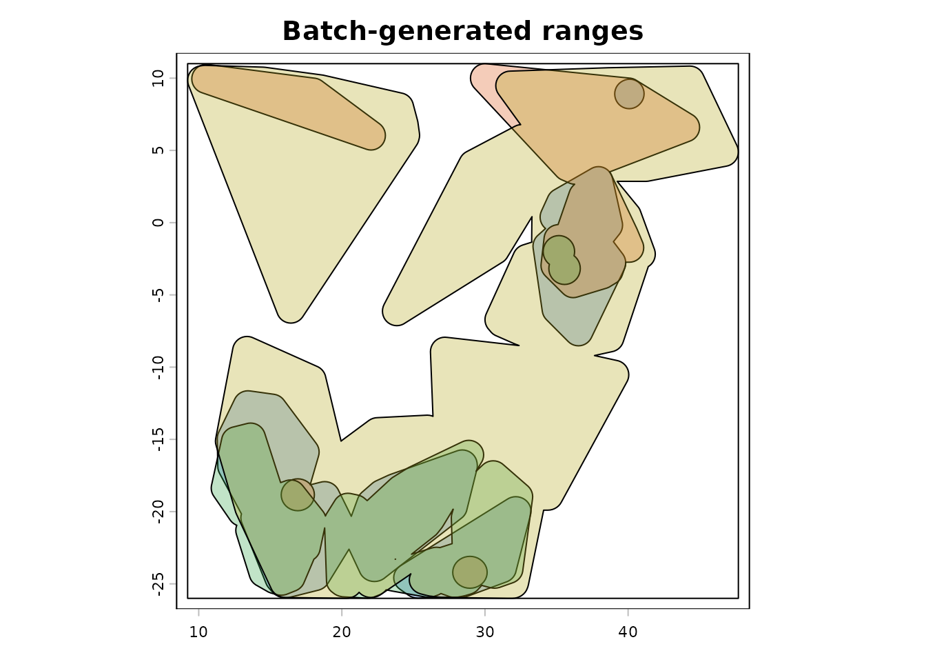
#> [1] "terra"

The example below overlays every saved range in the batch summary. This is a useful diagnostic pattern when checking whether a batch run produced geometries with the expected extent and shape.

range_colors <- c(
  rgb(0.10, 0.40, 0.75, 0.30),
  rgb(0.85, 0.35, 0.10, 0.30),
  rgb(0.20, 0.65, 0.30, 0.30),
  rgb(0.70, 0.65, 0.10, 0.30)
)

combined_ext <- terra::ext(first_range$rangeOutput)

if (nrow(range_summary) > 1) {
  for (i in 2:nrow(range_summary)) {
    range_i <- read_range_rds(range_summary$range_file[i])
    combined_ext <- terra::ext(
      min(terra::xmin(combined_ext), terra::xmin(range_i$rangeOutput)),
      max(terra::xmax(combined_ext), terra::xmax(range_i$rangeOutput)),
      min(terra::ymin(combined_ext), terra::ymin(range_i$rangeOutput)),
      max(terra::ymax(combined_ext), terra::ymax(range_i$rangeOutput))
    )
  }
}

terra::plot(combined_ext, col = NA, legend = FALSE, main = "Batch-generated ranges")
terra::plot(first_range$rangeOutput, add = TRUE, col = range_colors[1])

if (nrow(range_summary) > 1) {
  for (i in 2:nrow(range_summary)) {
    range_i <- read_range_rds(range_summary$range_file[i])
    terra::plot(range_i$rangeOutput, add = TRUE, col = range_colors[i])
  }
}

Practical advice

The disk-based workflow is most useful in three situations.

First, when a direct in-memory call to get_gbif() is not appropriate because the project already relies on downloaded GBIF exports.

Second, when a large multi-species table needs to be checked, cleaned, or archived at the species level before range inference.

Third, when the same species-specific occurrence files need to be processed repeatedly with different get_range() settings, ecoregions, or evaluation schemes.

The third point matters scientifically, not just computationally. It makes parameter sensitivity analyses much cleaner, because you can rerun the same archived species files under alternative ecoregion layers or buffering choices without changing the underlying occurrence input.

Take-home message

The disk-based workflow turns gbif.range into a practical bridge between very large GBIF exports and species-level range inference. Instead of treating file splitting and range building as an external preprocessing step, Gbif.range provides a coherent, testable, and documented path from a downloaded GBIF table to saved species ranges on disk.